Fitting
Small Angle X-Ray Data – Alumina Powder
In
this tutorial you will fit small angle scattering data for an alumina polishing
powder using data from a constant wavelength synchrotron X-ray USAXS
instrument. You will use both a lognormal distribution of spherical particles
model and a unified Guinier-Porod model. The data
were collected from powders
spread onto sticky tape and covered with another layer of the same tape. The
data were corrected for background using data collected from two layers of
sticky tape. However, the sample thickness is not accurately known so the data are not
calibrated on an absolute scale.
If you have not done so already, start GSAS-II.
Step 1: read in the data file
1. If you have saved the GSAS-II project file from the Size Distribution tutorial, use File/Open project… menu item to retrieve the data; plots of the size distribution and the data will appear. Then go to Step 2: Set Limits. Otherwise, use the Import/Small Angle Data/from q (A-1) step X-ray QIE data file menu item to read the data file into GSAS-II. This read option is set to read three column small angle scattering data (SASD) as Q in Å-1, intensity and estimated standard deviation in intensity; there may be a header with metadata information in the front of this file. Change the file directory to SAfit/data to find the file; you will have to select the any file (*.*) filter to see it.
2. Select the alumina data.dat data file in the first dialog and press Open. There will be a Dialog box asking Is this the file you want? Press Yes button to proceed.
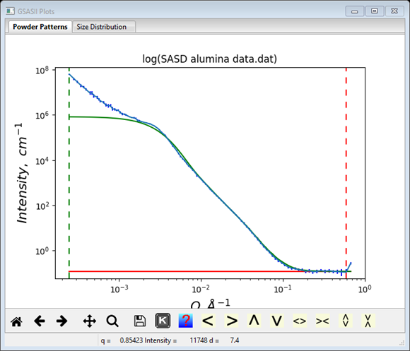
At this point the GSAS-II data tree window will have several entries and the plot window will show the SASD pattern as a log-log plot of intensity vs. Q
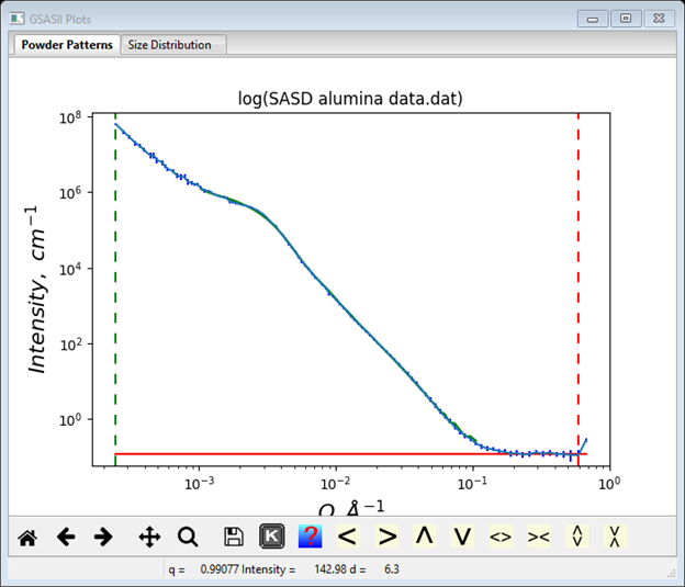
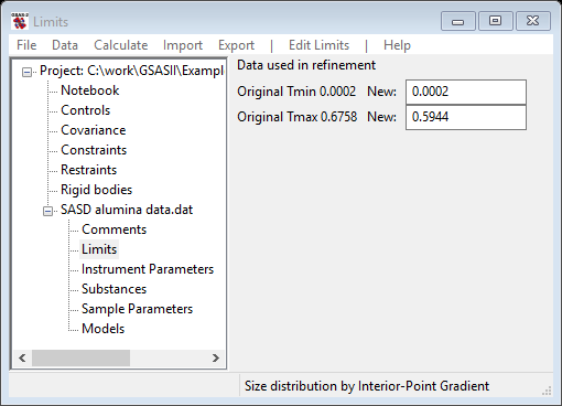
Step 2: Set Limits
For this step we will reposition the limits to exclude only the last point in the pattern as it does appear to be somewhat suspect (see plot). Select Limits under SASD alumina data.dat from the GSAS-II tree. Set the upper limit using the cursor on the plot by picking the next-to-last point on the curve with the left or right mouse button. If needed reposition the lower limit to be the 1st data point. The limits window should look like
Step 3 Select the scattering substances for your sample
If you have already done this step in the Size Distribution tutorial, skip to Step 4 Creation and Refinement of Log Normal Particle Model. Two substances need to be defined for your sample to give the anticipated scattering contrast; in this case one is alumina and the other is “vacuum” (really air). Parameters for a number of substances are defined in the file Substances.py. You can add your own substances to this or better put them in UserSubstances.py; this is read after Substances.py when you load substances for your selection. Select Substances under SASD alumina data.dat from the GSAS-II tree. Then do Edit substance/Load substance from the menu; a popup window will appear with possible selections
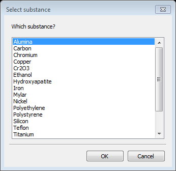
Select Alumina and press OK; the relevant data for alumina (and vacuum& unit scatter) are displayed next
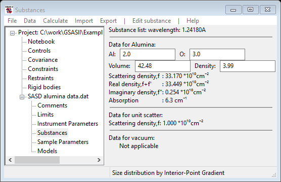
If desired you can load/add as many substances as you desire into this list; you can also delete any of them (except vacuum & unit scatter). The composition, volume occupied by the atoms in the composition and the density are given for each substance. These can each be edited; the other values will change accordingly. If your substance isn’t in the list, you can Edit substance/Add substance to create a new one (you will be asked for a name and the set of elements in two successive popup windows). From this information the scattering density and that as affected by resonant scattering for the listed wavelength is displayed (the wavelength can be changed in the Instrument Parameters GSAS-II tree item if needed). The resonant scattering value is used for contrast calculations.
Step 4 Creation and Refinement of Log Normal Particle Model
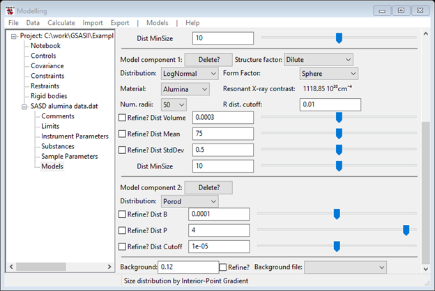
You are now ready to attempt fitting the data with a log normal distribution of spherical particles. Thus you’ll need to select Models under SASD alumina data.dat from the GSAS-II tree; the data window will display the Size dist. display; change this to Particle fit using the Modeling by pull down. NB: GSAS-II will remember your selection the next time you enter this Models data tree item.
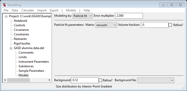
If you had done the Size Distribution tutorial, you would know that there were two populations of particles in the sample. One had a mean diameter of ~1300A and the other had a mean diameter of ~150A. You will also need something to describe the very lowest Q portion of the data. Do Models/Add from the menu; the data window will change and the plots will be refreshed. Your first step is to change the Material to Alumina and make sure the Background is something reasonable (0.12) based on the data at highest Q; again the data window and plots will be refreshed. Click on one of the slider buttons to force a calculation.
The data plot shows a horizontal red line for the background and a green one calculated from your selected model.

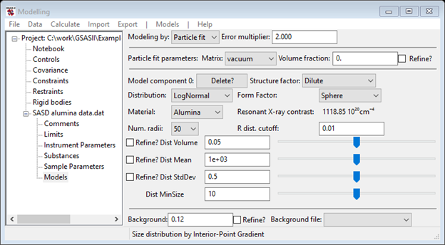
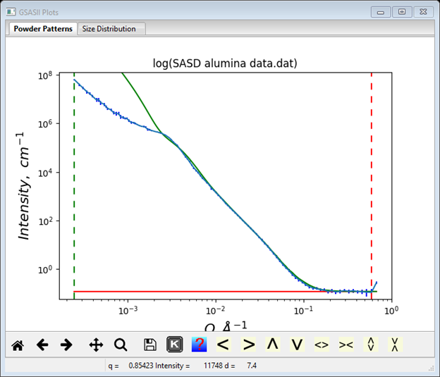
You can manually adjust the calculated curve by using the sliders: increase Dist Volume and decrease Dist Mean to improve the fit. NB: The Dist Mean is a radius so its value is roughly ½ the Size Distribution result. The sliders cover 2 orders of magnitude; their range is reset if a value is entered in the value field. After changing Dist Mean to 700 and Dist Volume to 0.0953 my plot is

There is an obvious discrepancy at low Q and a much less obvious one at Q~0.03-4Å-1; the latter is responsible for the ~150Å peak in the Size Distribution result. Do another Models/Add to include it. The data window now shows two components
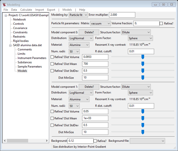
Note the Material for the new one is preset to Alumina to save you the easily forgotten step of setting it. Change Dist Mean to 75 (i.e. ½ of 150) and reduce Dist Volume to make the green curve better match the data (you can inset ‘0’s in the value & play with the slider – something like 0.0003 looks good). My fit looked like
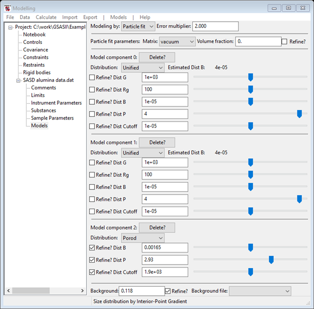
Finally we need to deal with the low Q region – this is probably due to some agglomeration of the 1300Å articles which is best described by a pure Porod power law scattering model. Do another Models/Add and change the Distribution selection to Porod. The third component is then (I’ve shrunk the window & moved the scroll bar).
The green curve on the plot looks very poor

Not to worry, all the problem is in the Porod component variables. Remembering that this is likely to be an agglomeration of 1300Å particles; set the Dist Cutoff to that value. That immediately restores the higher Q portion of the fit.
Next use the Dist P (power law exponent) slider to adjust the fit. In this case setting Dist P to ~3.25 gives a pretty good fit without needing to adjust the Dist B prefactor.
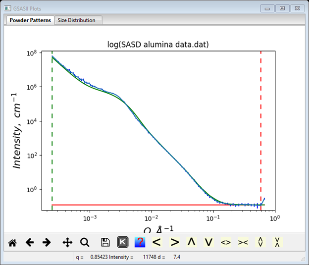
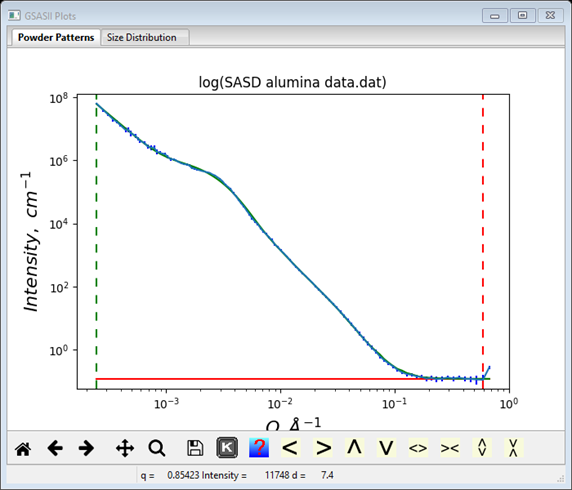
Finally, you can refine these coefficients to find the best fit to the data. As a beginner, I’d start by refining just the two Dist Volume and the Dist B along with the Background parameter (one might be able to refine “everything” at once, but then again it might not work). Check the Refine? boxes for these parameters. Do Models/Fit to do the least squares refinement; convergence will occur very quickly. NB: if the refinement messes up, you can recover the previous result; do Models/Undo to recover. Then add the two Dist Mean and Dist P parameters to the refinement, again convergence is easily obtained. Finally, add the two Dist StdDev and Dist Cutoff parameters (a total of ten) to the list. The result is a really nice fit to the data with reasonable values; the console window shows the full results of the refinement

If you had done a Size Distribution analysis, these results are plotted as component curves on that plot as well
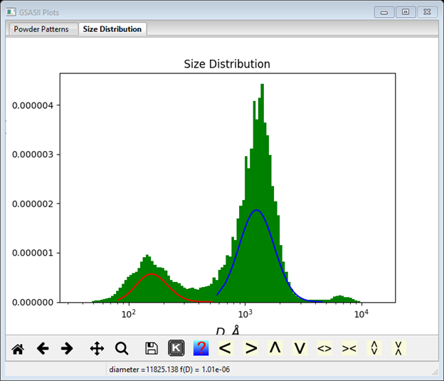
This is the sort of agreement one should expect between the best log normal fit and the size distribution. To save these results you must do File/Save project in the main GSAS-II data tree menu.
Step 6 Creation of a Unified Guinier-Porod Model
For the Unified model there is assumed to be particles with some radius of gyration (Guinier model) with a power law distribution tail (Porod model). This can be set for your model by changing the Distribution for the first two components to Unified. NB: the log normal coefficients are not lost by this step; they can be recovered by simply changing the Distribution back to LogNormal. The data window values give the defaults for these components
And the plot shows a poor fit

First, change the Dist Rg values to be about ½ the Size Distribution results (e.g. 700 & 75), then set the Dist Cutoff value for the Dist Rg=700 one to 100. Next, change the Dist G for the Dist Rg=700 one to be about the Intensity value for the lower Q bump in the data (~1.0e6). Finally, reduce the Dist G value for the Dist Rg=75 component to get the best fit to the data (~210). The data window looks like

And the plot looks like

This is probably close enough to do a refinement. Select Refine? For Dist G, Dist Rg and Dist B for both components (the Dist B, Dist P and Background Refine? boxes should also be checked). Then do Models/Fit; it should rapidly converge to give in the console window

And the closeness of the fit to the data in the plot is

This fit is almost as close as the log normal one done earlier. However, the Dist Rg values are a bit less than the corresponding Dist Mean values obtained earlier. Also note that this model makes no reference to the substance contrast used earlier (the Size Distribution plot will not have curves calculated from this model). To save these results you must do File/Save project in the main GSAS-II data tree window.
This concludes the SASD modeling tutorial.